Pseudo tiling of rasters
I am currently working on a project that involves machine learning to predict of ecological attributes across landscapes at fine spatial resolution. Our current list is consists of 80 covariates stacked together. To make predictions across the landscape significant tiling of the raster data is needed. However, the tiling process itself takes significant time and creates a tiled dataset in the thousands of tiles… There is another way!
Below I use two packages to create pseudo-tiles of the data.
GSIF::getSpatialTilesis used to generate a polygon layer of tiles covering the area of interest.STARS::read_starscan be used to load only a specific portion of each raster in the dataset.
library(tidyverse)
library(sf)
library(rgdal)
library(stars)
library(GSIF)
library(tmap)
Step 1: Define the tiles
Locate the data
I have previously confirmed that all of these layers stack (i.e. raster::stack(cv_list))
## list of rasters
  cv_list <- list.files("e:/tmpGIS/PEM_cvs/", pattern = "*.tif",full.names = TRUE)
  # cv <- list.files("c:/tmp", pattern = "*.tif", full.names = TRUE)
  cv_list <- cv_list[-(grep(cv_list, pattern = "xml"))] ## drop any associated xml files
  print(paste("there are", length(cv_list), "covariates in the list"))
## [1] "there are 80 covariates in the list"This next section is an adaptation of code provided by Tom Hengl.
## make tiles
  # GSIF requires a GDAL object
  cv1 <- GDALinfo(cv_list[1]) ## just loads the header info
  p_tiles <- GSIF::getSpatialTiles(cv1, block.x = 1000, return.SpatialPolygons = TRUE)
  p_tiles <- st_as_sf(p_tiles) %>% mutate(id = row_number())
  # Create tabular description of tiles -- generates a table of the extents of each tile
  t_tiles  <- GSIF::getSpatialTiles(cv1, block.x = 1000, return.SpatialPolygons = FALSE) %>%
    mutate(id = row_number())

  p_tiles <- left_join(p_tiles, t_tiles)
The attribute data provides all the information needed to generate a pseudo-tile.
head(as.data.frame(p_tiles) %>% dplyr::select(-geometry))## id xl yl xu yu offset.y offset.x region.dim.y region.dim.x
## 1 1 552600 5983800 553600 5984800 4820 0 400 400
## 2 2 553600 5983800 554600 5984800 4820 400 400 400
## 3 3 554600 5983800 555600 5984800 4820 800 400 400
## 4 4 555600 5983800 556600 5984800 4820 1200 400 400
## 5 5 556600 5983800 557600 5984800 4820 1600 400 400
## 6 6 557600 5983800 558600 5984800 4820 2000 400 400Step 2: Load Pseudo-tile
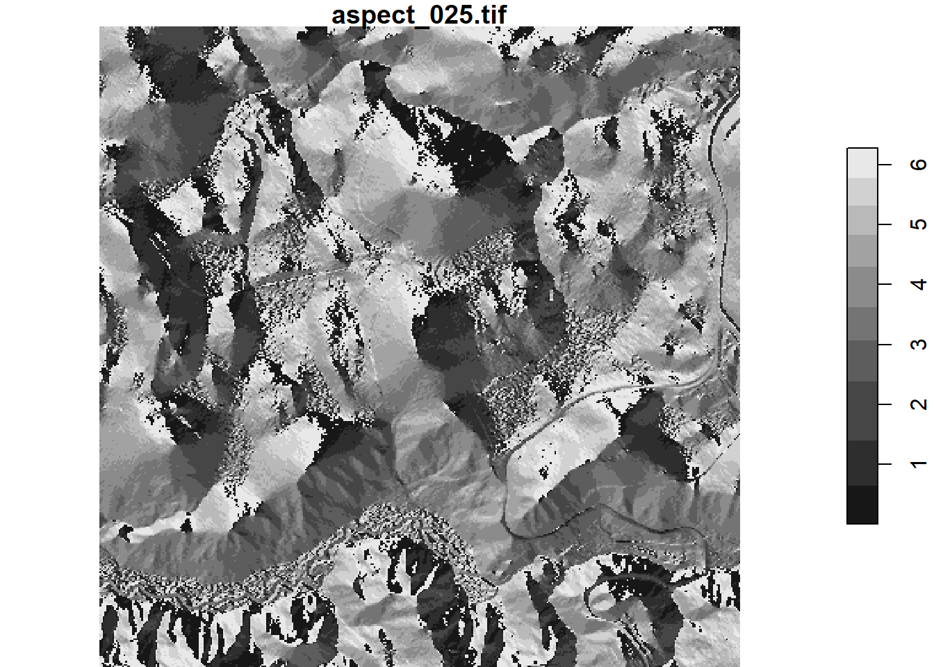
So other then defining what the tiles should be no tiles have actually been created. Now with the use of the stars package a tile can be loaded by specifying the pixel locations within the raster. Below tile number 167 is loaded
r <- read_stars(cv_list,
                RasterIO = list(nXOff  = t_tiles[167, "offset.x"],
                                nYOff  = t_tiles[167, "offset.y"],
                                nXSize = t_tiles[167, "region.dim.x"],
                                nYSize = t_tiles[167, "region.dim.y"]))
plot(r[1])
Figure 1: A tile extracted from a list of 80 covariate rasters
Next steps
Modeling
For modeling a stars object can be simply converted to a data.frame, be passed to a model, and then returned to the stars object. Hmmmn … not sure these steps are even needed … might be able to pass the object directly to a model. If not then the below will work.
df.r <- as.data.frame  ## convert to data.frame
df.r$uniform <- runif(nrow(df.r))  ## create a new attribute
r$uniform <- df.r$uniform  ## assign the attribute back to the stars object.
Build function
done!
I added tile_index() to the PEMgeneratr package. It takes a raster, and produces tiles of a specified pixel count (x by y). Here is an example:
t <- PEMgeneratr::tile_index(cv_list[1], 1000)

map <- tm_shape(t) + tm_polygons(alpha = 0.25)
tmap_leaflet(map)
my definition.↩