Using SuperLearner for Predictive Mapping
Recently I had the opportunity to attend a machine learning workshop hosted by the provincial BEC Team in Victoria, BC. and led by Tom Hengl of the OpenGeoHub Foudation. During this workshop we worked through various R machine learning packages. I learned some great new skills. The challenge really came down to taking time to understand all the steps – and then to apply it to my data / my projects.
Now that I have been able to take some time to mentally digest what I learned in Victoria this post provides a review of how to use the R SuperLearner package, to create predictive maps some of my data1.
SuperLearner
SuperLearner is an algorithm that uses cross-validation to estimate the performance of multiple machine learning models, or the same model with different settings. It then creates an optimal weighted average of those models, aka an “ensemble”, using the test data performance. This approach has been proven to be asymptotically as accurate as the best possible prediction algorithm that is tested.
( – Guide to SuperLearner)
Classification with SuperLearner
What I have come to understand in pulling this script together is that classification of discrete classes needs to be done step-wise. Here I mean that the training data needs to be converted to a binary question: Is this pixel part of ecotype_X?. Each discrete class is to evaluated individually. A composite map of all classes can be generated at the end using raster calculations … the easiest being raster::which.max().
Main steps
- Data needs
- geo-located training data
- co-variate raster data
- Convert data to a binary question (TRUE/FALSE)
- Provide an estimate of which methods and resulting ensemble using
CV.SuperLearner - Generate SuperLeaner model 4, Predict with SuperLearner model across the landscape
Packages/ libraries needed
## Libaries -------------------------------------------------
    ls <- c("tidyverse", "knitr")            # Data Management and Manipulation
    ls <- append(ls, c("sp", "GSIF"))        # geo comp.
    ls <- append(ls, c("rgdal", "sf", "raster", # more geo comp.
                       "rasterVis", "tmap", "RColorBrewer"))
    ls <- append(ls, "SuperLearner")

    ## additional needed libraries -- to be loaded as needed.
    ## library (snow)
    ## library (parallel)

## Install if needed -- then load.
    new.packages <- ls[!(ls %in% installed.packages()[,"Package"])]
    if(length(new.packages)) install.packages(new.packages)
    lapply(ls, library, character.only = TRUE)  # load the required packages
    rm(ls, new.packages)
Data
Data from the forest, the empircal data, is coupled with and raster layers which, through modeling we hope to use to predict real world values across the area of interest (aoi). In modeling terms the empirical data is the response variable and the raster layers are the predictive variables or covariates.
Below all the input data needed for this example is loaded.
## Load the training data -- 1st column is the response var, rest are predictor
dat <- read.csv("e:/workspace/2019/PEM/GITHUBv/PEM_Research_BC/ALRF/PEM_v2/data/train_data_clean.csv")

## raster data -- we will use these later for map generation
cv <- list.files("e:/tmpGIS/PEM_cvs/", pattern = "*.tif",full.names = TRUE)
# cv <- list.files("c:/tmp", pattern = "*.tif", full.names = TRUE)
cv <- cv[-(grep(cv, pattern = "xml"))] ## drop any associated xml files
cv <- stack(cv)
dim(cv)
## [1] 5220 6100 80Note that the raster stack is massive – this will prove problematic later. Trying to bring it into memory (i.e. using rgdal::readGDAL) attempts to create an object of 19Gb in size … a little beyond my laptop
Training and validation
The process to create training and validation datasets is quite straight forward (see the Guide to SuperLearner).
Is hold-back validation data needed when the modeling process provides cross validation?
The question is now binary: yes/no, true/false, with regard to is the data part of SBSwk1_01
Model Set up
Convert the question to a binary one
outcomes <- dat[,2]
table(outcomes)
## outcomes
## SBSwk1_01 SBSwk1_05 SBSwk1_06 SBSwk1_07 SBSwk1_08 SBSwk1_09 SBSwk1_11 SBSwk1_78
## 118 31 9 18 37 54 24 65
## SBSwk1_Wb sub-xeric xeric
## 30 13 9Currently, I have outcomes that will be used to predict 11 discrete classes as present above. These need to be converted to 11 individual classifications. For an example let’s predict one of the most common classes SBSwk1_01.
outcomes_bin <- as.numeric(outcomes == "SBSwk1_01")
table(outcomes_bin)
## outcomes_bin
## 0 1
## 290 118Machine Learners
SuperLearner supports numerous learners use listWrappers() to view them. For this example I have chosen:
- SL.caret.rpart
- SL.ranger (a re-write of randomForest)
- SL.svm – Support vector machine
- SL.mean – Effectively no model – used for a baseline (should be the worst performer)
sl <- c("SL.caret.rpart", "SL.ranger", "SL.svm", "SL.mean")Cross-validated risk estimate: CV.SuperLearner()
This function is used to provide an estimate of how well all the models being tested and the ensemble of all of them perform. The models are executed within a parallel processing framework using the snow package
modelName <- paste0("e:/workspace/tmp/SuperLearner/", "SiteSeries01", ".rds")
## if statement -- don't run the model if it has already been done
if(!file.exists(modelName)) {  ## if statement -- skip generation if it already exists
  ## Create Function
  # sl_MultiCV <- function(y_train = y_train, x_train = x_train){
      library(snow)
      cluster = parallel::makeCluster(parallel::detectCores()/2) # use half cores
      parallel::clusterEvalQ(cluster, library(SuperLearner))
      #parallel::clusterExport(cluster, learners$names) sent additional functions it they exist
      parallel::clusterSetRNGStream(cluster, 1) ## multicore type seed

      # with snow setup run the model
      system.time({
        cv_sl = CV.SuperLearner(Y = outcomes_bin, X = dat[, -c(1:2)],
                                family = binomial(), ## use binomial for single classes
                                # For a real analysis we would use V = 10.
                                V = 3,
                                parallel = cluster,
                                SL.library = sl
                                  )
      })
      parallel::stopCluster(cluster)
      # return(cv_sl) ## Turn on when converted to function.
  #} CLOSE FUNCTION
## Save the model object
saveRDS(cv_sl, modelName)
} else {
  cv_sl <- readRDS(modelName)
}
summary(cv_sl)
##
## Call:
## CV.SuperLearner(Y = outcomes_bin, X = dat[, -c(1:2)], V = 3, family = binomial(),
## SL.library = sl, parallel = cluster)
##
## Risk is based on: Mean Squared Error
##
## All risk estimates are based on V = 3
##
## Algorithm Ave se Min Max
## Super Learner 0.19243 0.0094159 0.17564 0.21712
## Discrete SL 0.20090 0.0100020 0.17487 0.24185
## SL.caret.rpart_All 0.21814 0.0117941 0.18647 0.24185
## SL.ranger_All 0.18899 0.0094093 0.17487 0.20611
## SL.svm_All 0.20447 0.0100559 0.18402 0.24147
## SL.mean_All 0.20901 0.0096770 0.18647 0.24185plot(cv_sl) + theme_minimal()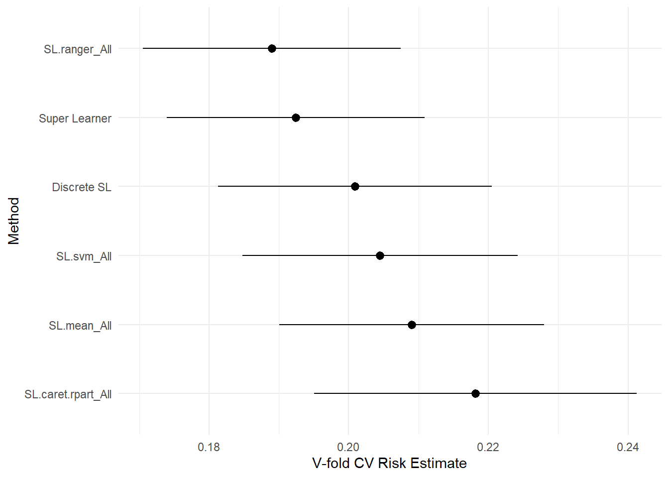
Cross-validated risk estimate: CV.SuperLearner() – take 2
Set hyper-parameters
The results show that ranger (aka randomForest) performs the best – distinctly outperforming the other models. However, how do other versions of `ranger compare when changing the hyperparameters?
below additional learners are created.
- Adjusting the number of trees within the random forest giving us four options to compare: using 250, 500 (default), 1000, and 2000trees.
- Adjusting the number of variables to split at each tree node is compared:
## Create Modifications to ranger's hyperparameters

myRanger_250 <- create.Learner("SL.ranger", params = list(num.trees = 250),
                               name_prefix = "Ranger250_trees")

myRanger_500 <- create.Learner("SL.ranger", params = list(num.trees = 500),
                               name_prefix = "Ranger500_trees")

myRanger_1000 <- create.Learner("SL.ranger", params = list(num.trees = 1000),
                               name_prefix = "Ranger1000_trees")

myRanger_2000 <- create.Learner("SL.ranger", params = list(num.trees = 2000),
                               name_prefix = "Ranger2000_trees")


## Comparing var splits at nodes
# Let's try 3 multiplies of this default: 0.5, 1, and 2.
(mtry_seq = floor(sqrt(ncol(dat[,-c(1:2)])) * c(0.5, 1, 2)))
## [1] 4 8 16myRanger_mtrys <- create.Learner("SL.ranger", tune = list(mtry = mtry_seq),
name_prefix = "Ranger500_mtrys")
myRanger_1000_mtry4 <- create.Learner("SL.ranger", params = list(num.trees = 1000,
mtry_seq = 4),
name_prefix = "Ranger1000_trees_mtry4")Estimate of risk: CV.SuperLearner
The variations of SL.ranger along with SL.mean (for comparison) are tested.
Note the additional sending of these learners above to the multicore process
## Create vector of SuperLearners to use
# sl2 <- c("my.ranger.250t", "SL.ranger", "my.ranger.1000t", "my.ranger.2000t", "SL.mean" )
sl2 <- c(myRanger_250$names, myRanger_500$names, myRanger_1000$names,
         myRanger_2000$names, myRanger_mtrys$names, myRanger_1000_mtry4$names,
         "SL.svm",  "SL.mean")

sl2
## [1] "Ranger250_trees_1" "Ranger500_trees_1"
## [3] "Ranger1000_trees_1" "Ranger2000_trees_1"
## [5] "Ranger500_mtrys_1" "Ranger500_mtrys_2"
## [7] "Ranger500_mtrys_3" "Ranger1000_trees_mtry4_1"
## [9] "SL.svm" "SL.mean"modelName <- paste0("e:/workspace/tmp/SuperLearner/", "SiteSeries_rangers_01", ".rds")
## if statement -- don't run the model if it has already been done
if(!file.exists(modelName)) { ## if statement -- skip generation if it already exists
## Create Function
# sl_MultiCV <- function(y_train = y_train, x_train = x_train){
library(snow)
cluster = parallel::makeCluster(parallel::detectCores()-2) # use half cores
parallel::clusterEvalQ(cluster, library(SuperLearner))
## IMPORTANT!! send additional learners to cluster -----------
parallel::clusterExport(cluster, myRanger_250$names)
parallel::clusterExport(cluster, myRanger_500$names)
parallel::clusterExport(cluster, myRanger_1000$names)
parallel::clusterExport(cluster, myRanger_2000$names)
parallel::clusterExport(cluster, myRanger_mtrys$names)
parallel::clusterExport(cluster, myRanger_1000_mtry4$names)
## Set seed -- common seed for all cores
parallel::clusterSetRNGStream(cluster, 1) ## multicore type seed
# with snow setup run the model
system.time({
cv_sl = CV.SuperLearner(Y = outcomes_bin, X = dat[, -c(1:2)],
family = binomial(), ## use binomial for single classes
# For a real analysis we would use V = 10.
V = 3,
parallel = cluster,
SL.library = sl2
)
})
parallel::stopCluster(cluster)
# return(cv_sl) ## Turn on when converted to function.
#} CLOSE FUNCTION
## Save the model object
saveRDS(cv_sl, modelName)
} else {
cv_sl <- readRDS(modelName)
}
summary(cv_sl)##
## Call:
## CV.SuperLearner(Y = outcomes_bin, X = dat[, -c(1:2)], V = 3, family = binomial(),
## SL.library = sl2, parallel = cluster)
##
## Risk is based on: Mean Squared Error
##
## All risk estimates are based on V = 3
##
## Algorithm Ave se Min Max
## Super Learner 0.18604 0.0092195 0.16623 0.21043
## Discrete SL 0.18513 0.0094466 0.16167 0.21171
## Ranger250_trees_1_All 0.18571 0.0098682 0.16320 0.21003
## Ranger500_trees_1_All 0.18687 0.0096919 0.16427 0.21352
## Ranger1000_trees_1_All 0.18570 0.0096900 0.16261 0.21156
## Ranger2000_trees_1_All 0.18586 0.0097594 0.16315 0.21163
## Ranger500_mtrys_1_All 0.18610 0.0094894 0.16457 0.21171
## Ranger500_mtrys_2_All 0.18669 0.0097556 0.16331 0.21265
## Ranger500_mtrys_3_All 0.18651 0.0098626 0.16381 0.21135
## Ranger1000_trees_mtry4_1_All 0.18502 0.0096838 0.16167 0.21060
## SL.svm_All 0.19438 0.0098584 0.18525 0.21244
## SL.mean_All 0.20635 0.0095204 0.19599 0.22151plot(cv_sl) + theme_minimal()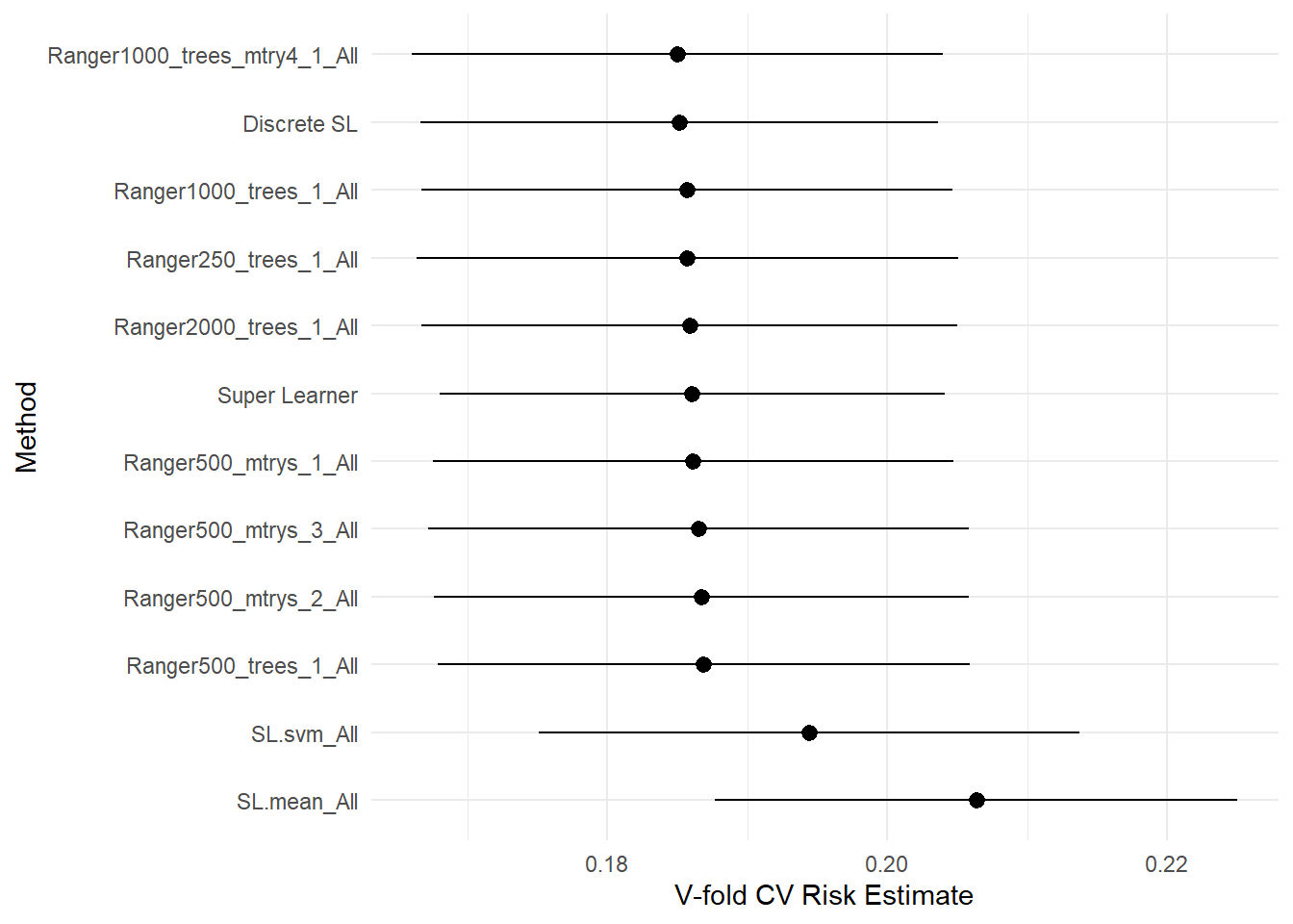
Generation of model: snowSuperLearner
Based on the above the default settings of ranger performed the best – though given sd bars likely no real difference with changes to hyperparameters.
As such I am going to generate a model using just that package. Note that SuperLearner’s ensemble was marginally lower than ranger as the other models actually pulled its results down.
## Specify sl's to use
sl3 <- "SL.ranger"

modelName <- paste0("e:/workspace/tmp/SuperLearner/", "SiteSeries_ranger_model_01", ".rds")

if(!file.exists(modelName)){
## the next execution has potential conflicts with the snow package
detach("package:snow", unload=TRUE)


  library(parallel)
  system.time({
    cluster <- parallel::makeCluster(detectCores()-2)
    x <- parallel::clusterEvalQ(cluster, library(SuperLearner))  ## pass these to the multi-core process
    cv_sl_Prediction = snowSuperLearner(Y = outcomes_bin, X = dat[, -c(1:2)],
                           family = binomial(),
                           cluster = cluster,
                           SL.library = sl3,
                           # For a real analysis we would use V = 10.
                           cvControl=list(V=5))

  })
  saveRDS(cv_sl_Prediction, modelName)
} else {
   cv_sl_Prediction <- readRDS(modelName)
}
Predict across landscape
Tiling of rasters
As per the methods we learned in Victoria the data needs to be converted to a SpatialPointDataFrame. However, the current data set is much too large for this. Also, as emphasized in Victoria, this is where tiling of the raster becomes essential and to do that in parallel processing (while playing nice with the raster package)2.
… long story short – I ended up building a wrapper function for SPAdes.tools::splitRaster which generates all the tiles needed using parallel processing – and is friendly with the raster package. I did not include that here – it will be included in the PEMgeneratr package that is in development.
Load a tile
As an example here one tile is loaded.
For full implementation this should be completed within a loop cycling through all the tiles – and done in parallel.
## Figure out which tile to load
# tiles <- "e:/tmpGIS/PEM_cvs/tiles.gpkg"
# tiles <- st_read(tiles)
# mapview::mapview(tiles, zcol = "index", alpha = 0.5)

lt <- list.files("e:/tmp/cvs/tiles/aspect_025/", pattern = "tile109", full.names = TRUE)
lt <- lt[!grepl(".grd", lt)]

cv_tile <- stack(lt)
Convert to SpatialPixelDataFrame
system.time({
  spdf <- as(cv_tile, "SpatialPixelsDataFrame")
})
## user system elapsed
## 3.82 0.15 4.04plot(spdf[,"aspect_025"], main = "Aspect - 2.5m resolution")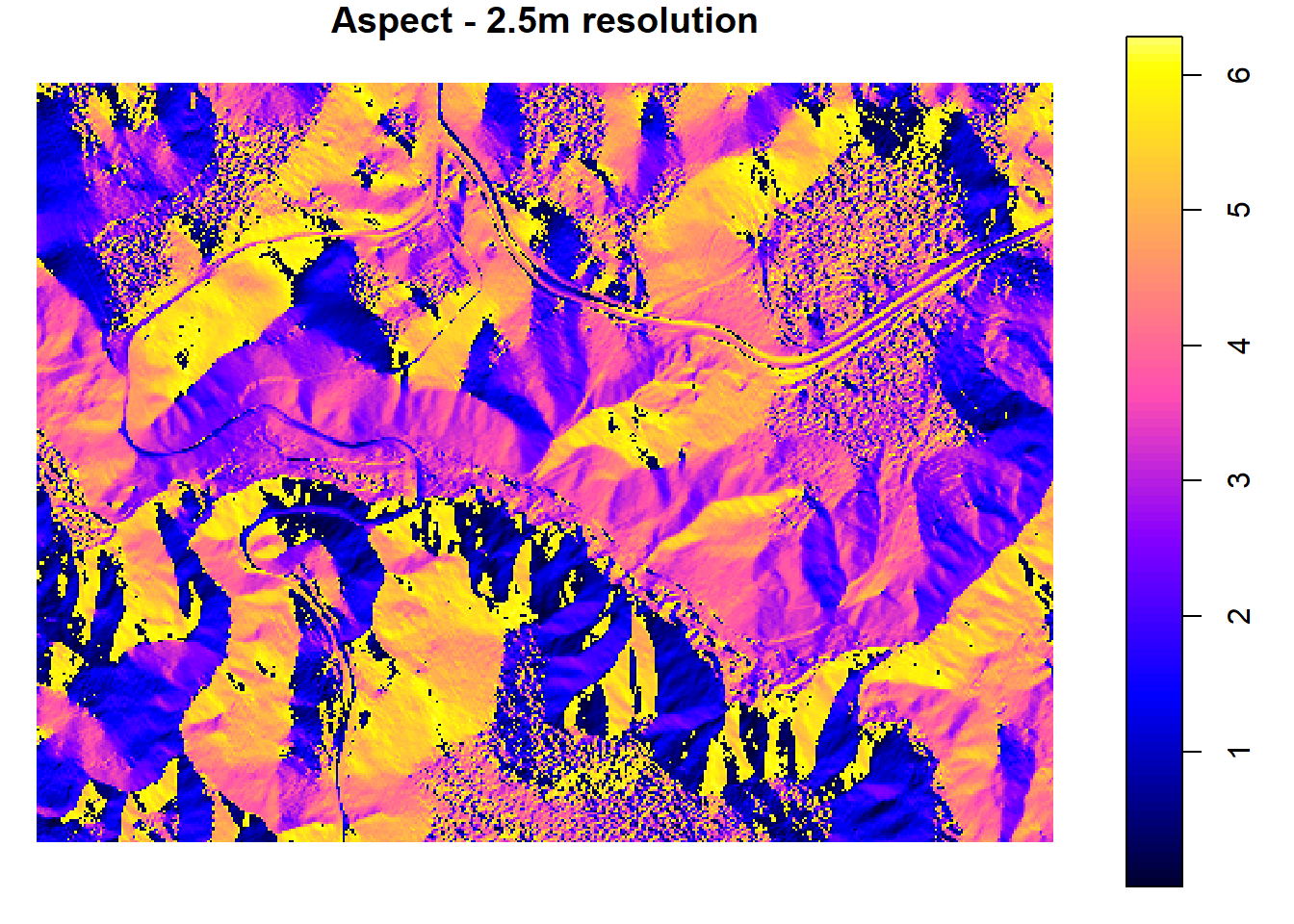
Apply Prediction
Now all the data can be accessesed and sent through the model generated above.
tileOut <- "./SBSwk1.tif"
if(!file.exists(tileOut)){  ## if prediction is generated don't do it again.
new.data <- spdf@data ## just the data is used (as a data.fame)

## prediction data is generated
pred <- predict(cv_sl_Prediction, new.data[,cv_sl_Prediction$varNames])

## prediction data is applied to raster
spdf@data[,"SBSwk1_01"] <- pred ## puts the data back into the spatial dataframe -- as a new column
r <- raster(spdf[,"SBSwk1_01"])
writeRaster(r, tileOut)
} else {
  r <- raster(tileOut)
}


my_pal <- colorRampPalette(brewer.pal(100, "Greens"))
my_pal <- my_pal((100))
plot(r, main = "Probability of 'SBSwk1_01'", col = my_pal)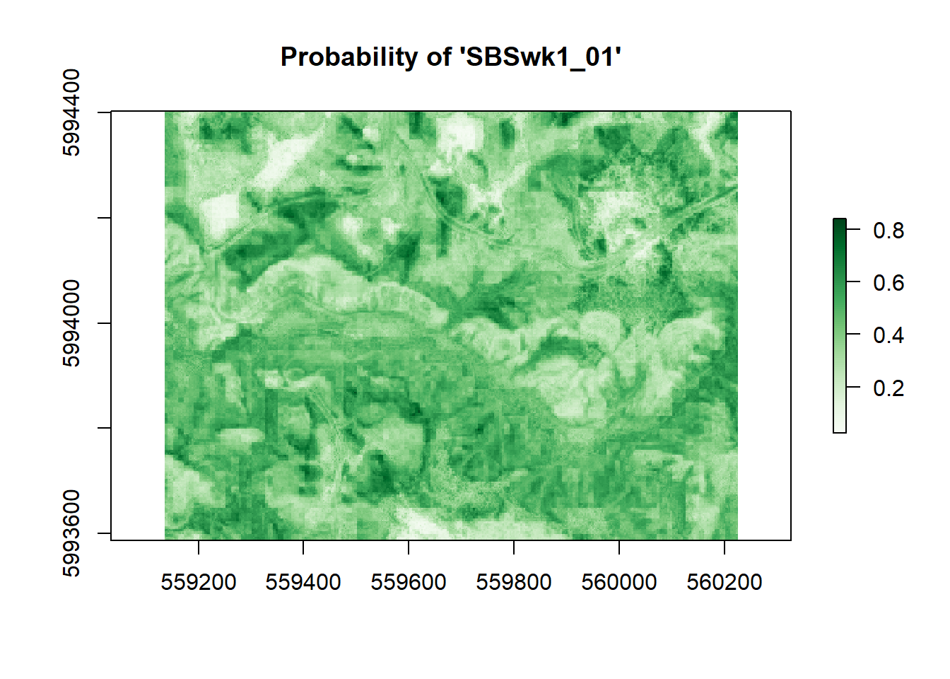
Additional resources
More toys to try (found these while trying to solve issues in building the above).
- https://rpubs.com/erobinson95/superlearner. provides more detail on optimizing hyper parameters.
- see the
caretpackage as many of the learners are the same. - https://cran.r-project.org/web/packages/TileManager/TileManager.pdf
- http://spades.predictiveecology.org/ – lots to explore here…
- https://cran.r-project.org/web/packages/gdalUtils/gdalUtils.pdf
for a fuller explaination see Hengl and MacMillan’s Predictive Soil Mapping with R↩
This process took about 2 hours … with a ferrari it would have taken more like 10-12mins – wishing I had a ferrari↩
Colin Chisholm
Professional Forester bridging the gap between the academic and operational worlds.