Using mlr for predictive mapping
In a previous post I used SuperLearner for Predictive Mapping. Here following guidance from Hefin Rhys’ youtube tutorial and some scripting made available by Tomislav Hengl of OpenGeoHub. I will demonstrate generating a ranger, random forest, model to predict multiclass and probability of each class. Data is currently closed but I hope to make it open down the road.
The mlr package (machine learning in r), is a package that acts as a wrapper for numerous machine learning algorithms. Using this package allows for accessing these different tools via a consistent syntax. There are a few key steps in generating a mlr model.
Load the Data
# install.packages("mlr", dependencies = TRUE)
library(mlr)
library(tidyverse)
library(sf)
library(rgdal)
library(raster)
library(stars)
library(GSIF)
library(tmap)
library(RColorBrewer)

## Load the data
modDat <- read.csv("e:/workspace/2020/PEM/ALRF_PEMv2/dev/modDat.csv",
                   stringsAsFactors = TRUE)  ## the var to be predicted needs to be a factor
# str(modDat)


## define output directory
outDir <- "e:/tmpGIS/R_mlr_post/"
Site Series calls
These are the ecosystem classes that we want to predict.
table(modDat$SiteSeries)##
## SBSwk1_01 SBSwk1_05 SBSwk1_06 SBSwk1_07 SBSwk1_08 SBSwk1_09 SBSwk1_10 SBSwk1_11
## 283 28 21 276 271 268 115 107
## sub-xeric Wb
## 17 16Step 1: Define a task
This simply declares the data set and the target to predict on. In this example I use data from the Aleza Lake Research Forest points are known site series and ecological classification using the province of British Columbia’s BEC Classification system. To create a predicted ecosystem model co-variate layers are used.
tsk <- makeClassifTask(data = modDat, target = "SiteSeries")Step 2: Define a learner
The learner is the algorithm that will be used to create the model, including specific parameters within the model
## STEP 2: Define a Learner --------
## maybe increase trees to 500 -- set to 100 for faster demonstration
  lrn <- makeLearner("classif.ranger",
                     num.trees = 100,                         ## number of trees DEFAULT: 500
                     mtry = round(sqrt(ncol(modDat)-1)),      ## someone showed me to declare mtry this way
                     num.threads = parallel::detectCores()*2, ## CAUTION HERE: how many threads does your machine have?
                     importance = "impurity",                 ## collect var importance data
                     predict.type = "prob")
All of the parameters available for any specific model can be listed by calling getLearnerParamSet(lrn). To view all the current parameter settings for a specific learner use getHyperPars(lrn)
  # getLearnerParamSet(lrn)  ## list all of the parameter settings available for the learner
  # getHyperPars(lrn)        ## list parameters set in learner)
Step 3: Validation
Best practice is to examine model performance. It seems counter-intuitive but this is done before the model is actually trained.
Define the resampling method
In this example I am using a repeated k-fold cross-validation.
  resp <- makeResampleDesc("RepCV",     ## repeated cross fold
                           folds = 5,   ## k-folds 5 or 10 as default
                           reps  = 3)   ## note this will mean 5 x 3 = 50 iterations through the data
     ## note: 5 fold 3 repeats is a little low.  I would prefer 10 x 10 but that takes additional time...
Perform validation
The following performs the resampling and provides a metric of performance: mean mis-classification error.
  cv <- mlr::resample(learner = lrn,
                 task = tsk,
                 resampling = resp)
Confusion matrix
To examine where misclassifications are occurring a confusion matrix is a great tool. Below two options are provided. First, a relative confusion matrix.
## calculate the confusion matrix
  cf_matrix <- calculateConfusionMatrix(cv$pred,
                                        relative = TRUE,
                                        sums = TRUE)
## Confusion matrix as relative ratio
round(cf_matrix$relative.row, 2)## SBSwk1_01 SBSwk1_05 SBSwk1_06 SBSwk1_07 SBSwk1_08 SBSwk1_09 SBSwk1_10
## SBSwk1_01 0.72 0.03 0.00 0.11 0.12 0.02 0.00
## SBSwk1_05 0.67 0.19 0.00 0.04 0.01 0.00 0.00
## SBSwk1_06 0.00 0.00 0.14 0.27 0.00 0.49 0.03
## SBSwk1_07 0.15 0.00 0.00 0.58 0.06 0.18 0.02
## SBSwk1_08 0.14 0.00 0.00 0.12 0.65 0.04 0.05
## SBSwk1_09 0.03 0.00 0.01 0.15 0.06 0.66 0.03
## SBSwk1_10 0.01 0.00 0.01 0.17 0.31 0.21 0.29
## SBSwk1_11 0.02 0.00 0.01 0.03 0.00 0.40 0.00
## sub-xeric 0.08 0.00 0.00 0.00 0.14 0.00 0.00
## Wb 0.00 0.00 0.00 0.00 0.00 0.38 0.00
## SBSwk1_11 sub-xeric Wb -err-
## SBSwk1_01 0.00 0.00 0.00 0.28
## SBSwk1_05 0.00 0.10 0.00 0.81
## SBSwk1_06 0.06 0.00 0.00 0.86
## SBSwk1_07 0.01 0.00 0.00 0.42
## SBSwk1_08 0.00 0.00 0.00 0.35
## SBSwk1_09 0.06 0.00 0.00 0.34
## SBSwk1_10 0.00 0.00 0.00 0.71
## SBSwk1_11 0.54 0.00 0.00 0.46
## sub-xeric 0.00 0.78 0.00 0.22
## Wb 0.48 0.00 0.15 0.85Second, a confusion matrix as total counts in each class and mis-classification.
  ## Confusion matrix all
  cf_matrix$result
## SBSwk1_01 SBSwk1_05 SBSwk1_06 SBSwk1_07 SBSwk1_08 SBSwk1_09 SBSwk1_10
## SBSwk1_01 613 22 0 91 103 16 2
## SBSwk1_05 56 16 0 3 1 0 0
## SBSwk1_06 0 0 9 17 0 31 2
## SBSwk1_07 124 0 3 481 50 147 16
## SBSwk1_08 114 0 0 96 528 31 41
## SBSwk1_09 22 0 5 120 51 529 26
## SBSwk1_10 5 0 2 60 107 72 99
## SBSwk1_11 6 0 2 9 1 130 0
## sub-xeric 4 0 0 0 7 0 0
## Wb 0 0 0 0 0 18 0
## -err.- 331 22 12 396 320 445 87
## -n- 944 38 21 877 848 974 186
## SBSwk1_11 sub-xeric Wb -err.- -n-
## SBSwk1_01 2 0 0 236 849
## SBSwk1_05 0 8 0 68 84
## SBSwk1_06 4 0 0 54 63
## SBSwk1_07 7 0 0 347 828
## SBSwk1_08 0 3 0 285 813
## SBSwk1_09 51 0 0 275 804
## SBSwk1_10 0 0 0 246 345
## SBSwk1_11 172 0 1 149 321
## sub-xeric 0 40 0 11 51
## Wb 23 0 7 41 48
## -err.- 87 11 1 1712 NA
## -n- 259 51 8 NA 1402Step 4: Train the model
Assuming that the metrics above is performing adequately the model can be trained. Note: I did not include an optional step for tuning the model hyperparameters.
train the model:
mod <- train(lrn, tsk)Variable importance
var_imp <- as.data.frame(mod$learner.model$variable.importance) %>%
    rownames_to_column()
  names(var_imp) <- c("name", "VaribleImportance")

var_imp %>% arrange(desc(VaribleImportance)) %>% head(., 10)
## name VaribleImportance
## 1 TWI_10m 33.31014
## 2 TWI_25m 28.47959
## 3 MRVBF_025 25.03336
## 4 MRVBF_10m 23.09211
## 5 Slope_10m 22.63159
## 6 TRI_05m 22.61561
## 7 MRVBF_05m 22.50482
## 8 p50_25m 21.44232
## 9 OpennessNegative_10m 18.27778
## 10 Slope_05m 18.14565Step 5: Predict
In this case as we are modelling across a landscape a raster stack is loaded.
Load raster data
See my Pseudo tiling of rasters post for a fuller description of loading large rasters.
## Figure out which tile to load
# tiles <- "e:/tmpGIS/PEM_cvs/tiles.gpkg"
# tiles <- st_read(tiles)
# mapview::mapview(tiles, zcol = "index", alpha = 0.5)

## list of rasters
  cv_list <- list.files("e:/tmpGIS/PEM_cvs/", pattern = "*.tif",full.names = TRUE)
  # cv <- list.files("c:/tmp", pattern = "*.tif", full.names = TRUE)
  cv_list <- cv_list[-(grep(cv_list, pattern = "xml"))] ## drop any associated xml files
  # print(paste("there are", length(cv_list), "covariates in the list"))
Create polygon tiles of the raster stack
## make tiles
  # GSIF requires a GDAL object
  cv1 <- GDALinfo(cv_list[1]) ## just loads the header info
  p_tiles <- GSIF::getSpatialTiles(cv1, block.x = 1000, return.SpatialPolygons = TRUE)
  p_tiles <- st_as_sf(p_tiles) %>% mutate(id = row_number())
  # Create tabular description of tiles -- generates a table of the extents of each tile
  t_tiles  <- GSIF::getSpatialTiles(cv1, block.x = 1000, return.SpatialPolygons = FALSE) %>%
    mutate(id = row_number())

  p_tiles <- left_join(p_tiles, t_tiles)
Load one of the tiles. The raster stack layer names are renamed, dropping the file extension, and thereby matching the modDat names.
r <- read_stars(cv_list,
                RasterIO = list(nXOff  = t_tiles[167, "offset.x"],
                                nYOff  = t_tiles[167, "offset.y"],
                                nXSize = t_tiles[167, "region.dim.x"],
                                nYSize = t_tiles[167, "region.dim.y"]))


## Rename the layer names (drop the .tif from the layer names)
r_names <- names(r)
r_names <- gsub(pattern = ".tif", "", r_names)
names(r) <- r_names

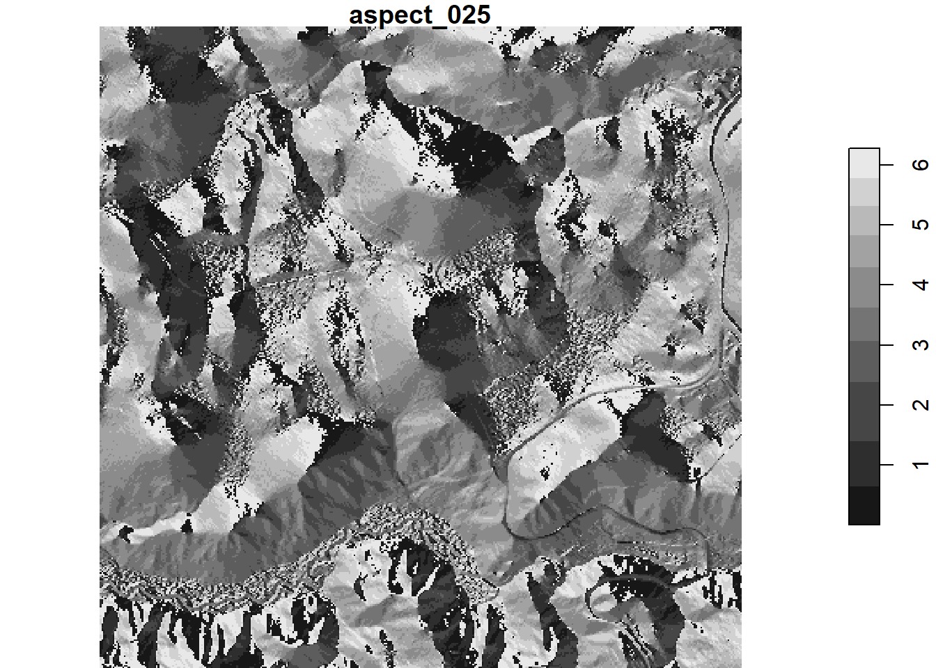
plot(r[1])
Predict using the raster data
Convert raster to sf data frame
The stars package allows for easy access to portions of a raster, (i.e. a specific window on the raster stack – see above). However, some data manipulation is needed to access the data in a data-frame format needed by mlr::predict().
## Converts STARS object to sf point object -- allows data.frame access.
r_spd <- st_as_sf(r,as_points = TRUE)
# st_bbox(r) == st_bbox(r_spd)

## Predicts the new values
pred <- predict(mod, newdata = r_spd)
The predicted values now need to be assigned to a raster. Here the predicted values are bound to the sf / data-frame re-establishing spatial geometry, and then that data frame is reduced to just the predicted values.
r_out <- cbind(r_spd, pred)
# r_out <- r_out[,length(r)+1:length(r_out)]

## layers to keep (i.e. newly predicted layers)
keep <- setdiff(names(r_out),
        names(r))
keep <- keep[-length(keep)] ## drops the last entry (geometry field, not a name)
keep
## [1] "prob.SBSwk1_01" "prob.SBSwk1_05" "prob.SBSwk1_06" "prob.SBSwk1_07"
## [5] "prob.SBSwk1_08" "prob.SBSwk1_09" "prob.SBSwk1_10" "prob.SBSwk1_11"
## [9] "prob.sub.xeric" "prob.Wb" "response"## layers / columns are reduced to just the
r_out <- r_out %>% dplyr::select(keep)One small house-keeping issue is that the multiclass prediction is a factor. This needs to be converted to numeric to facilitate conversion to raster.
## What the levels are in the multiclass
respNames <- levels(r_out$response) ## this becomes the dictionary to describe the raster values
respNames
## [1] "SBSwk1_01" "SBSwk1_05" "SBSwk1_06" "SBSwk1_07" "SBSwk1_08" "SBSwk1_09"
## [7] "SBSwk1_10" "SBSwk1_11" "sub-xeric" "Wb"## save the response names
write.csv(respNames, paste0(outDir, "response_names.csv"), row.names = FALSE)
## Convert to a numeric so that it can be rasterized
r_out$response <- as.numeric(r_out$response) ## convert to numericRasterize
Finally the sf object is converted to a set of rasters. So far it seems a loop is needed as st_rasterize only produces one raster at a time. Note that a template is specified ensuring that the output data matches the extent of the input data.
for (i in 1:length(keep)) {        ## -1 to skip the geom column
  # print(keep[i])
  out <- st_rasterize(r_out[,i],     ## specifies the specific layer
                      template = r)  ## uses the original raster as the template
  write_stars(out,
              dsn = paste0(outDir, keep[i], ".tif"))
}list.files(outDir)## [1] "prob.SBSwk1_01.tif" "prob.SBSwk1_05.tif" "prob.SBSwk1_06.tif"
## [4] "prob.SBSwk1_07.tif" "prob.SBSwk1_08.tif" "prob.SBSwk1_09.tif"
## [7] "prob.SBSwk1_10.tif" "prob.SBSwk1_11.tif" "prob.sub.xeric.tif"
## [10] "prob.Wb.tif" "response.tif" "response.tif.aux.xml"
## [13] "response_names.csv"Plot results
## list of rasters
  tifs <- list.files(outDir, pattern = "*.tif",full.names = TRUE)
  tifs <- tifs[!grepl("xml", tifs)]

siteSeries <- stack(tifs[-11]) ## note using raster stack here to facilitate plot, ignoring the multiclass for now
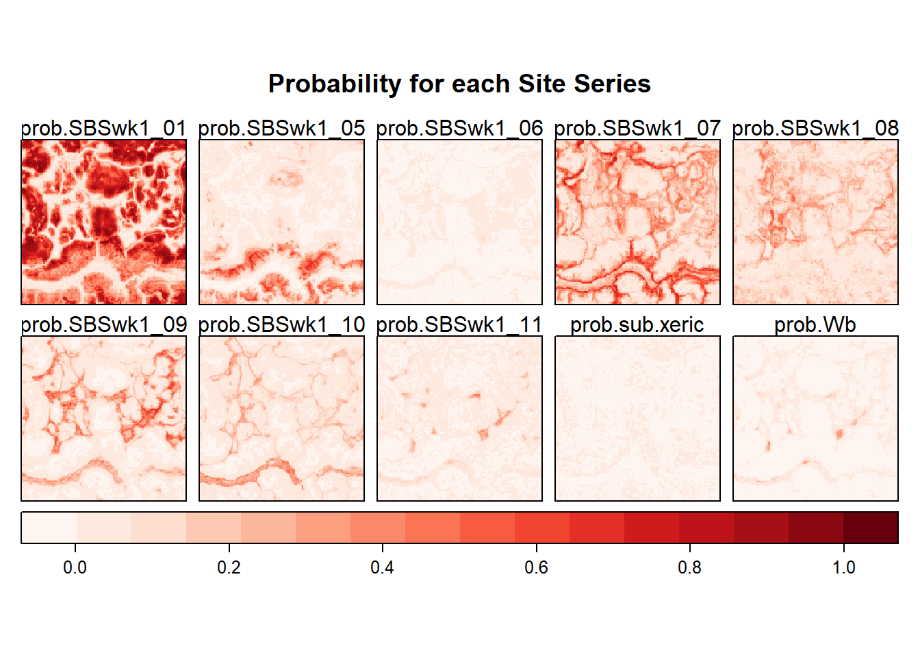
Probability Layers
my_pal <- colorRampPalette(brewer.pal(100, "Reds"))
my_pal <- my_pal((100))

rasterVis::levelplot(siteSeries,
          main = "Probability for each Site Series",
          layout = c(5, ceiling(length(names(siteSeries))/5)),
          col.regions=my_pal,
          scales=list(draw=FALSE ),
          colorkey=list(space="bottom"))
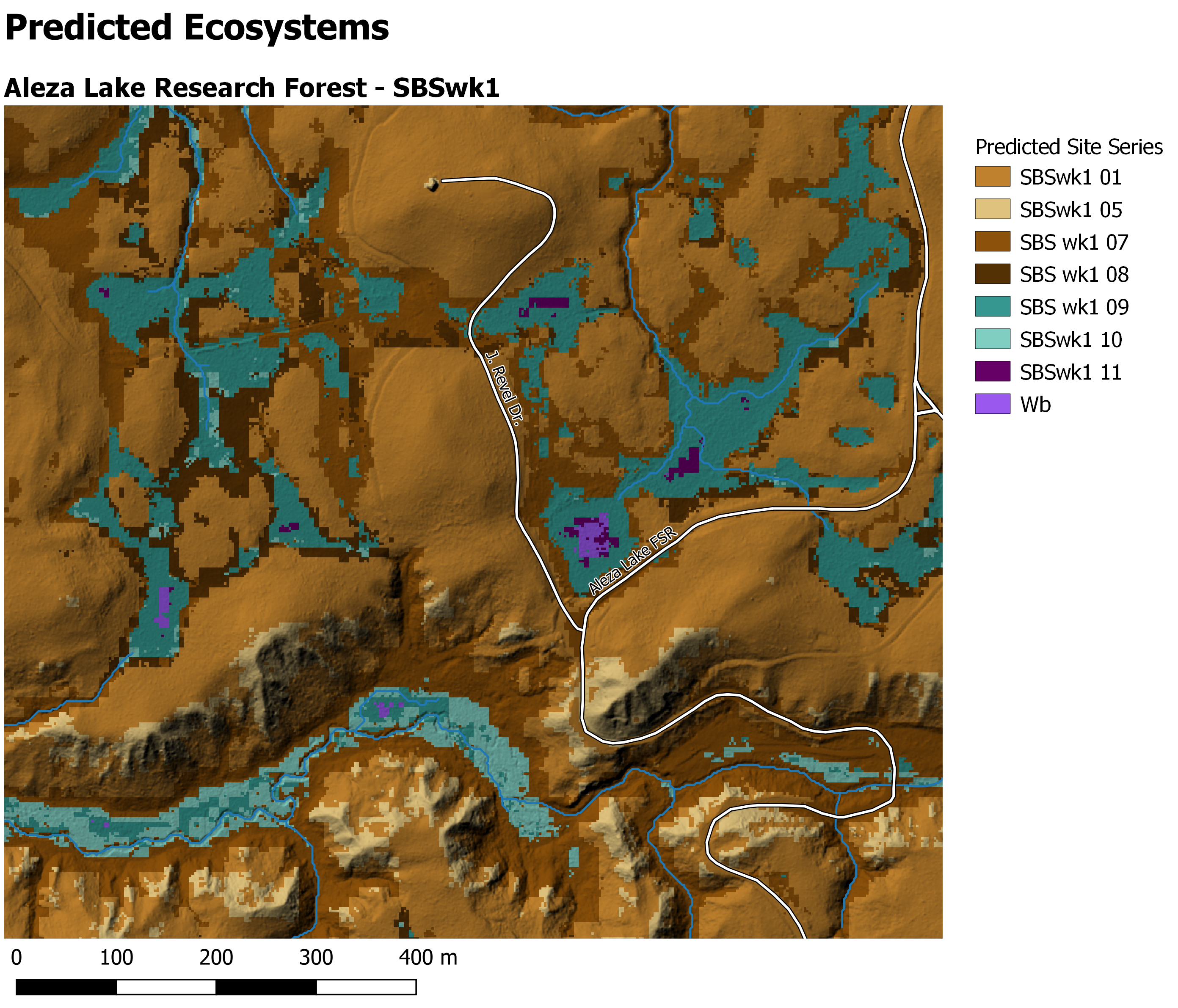
Multiclass
knitr::include_graphics("/img/PEMv2_tile.png")
Figure 1: Multiclass prediction of site series with hillshade. Note: map created in QGIS
Auto-generation map of multiclass
This generally worked… but needs some polish. Included for reference. What did not work is that the 06 site series was not predicted on this tile and so that messed up the coloration for all of the remaining site series.
## auto generated multi class
siteSeries <- raster(tifs[11])

## Prepare color palette
  legend <- respNames #; leg <- c("na", leg)
  brk <- seq(1:length(legend))
  # my_pal <- colorRampPalette(c("brown", "green", "blue"), space = "Lab")
  # # my_pal <- colorRampPalette(brewer.pal(length(legend), "BrBG"))
  # my_pal <- my_pal(length(legend))
  # # my_pal <- c("#000000", my_pal)

## manual color palette -- see: http://colorbrewer2.org/#type=diverging&scheme=BrBG&n=10
  my_pal <- c("#bf812d", ## 01
              "#dfc27d", ## 05
              "#c7eae5", ## 06
              "#8c510a", ## 07
              "#543005", ## 08
              "#35978f", ## 09
              "#80cdc1", ## 10
              "#01665e", ## 11
              "#f6e8c3", ## sub-xeric
              "#35978f" ## Wb
  )


## Plot Raster see: https://www.neonscience.org/raster-data-r
par(xpd = FALSE,mar=c(5.1, 4.1, 4.1, 4.5))
plot(siteSeries, col = my_pal,
       main = "Predicted Site Series",
       breaks = brk,  lab.breaks = brk,
       legend = FALSE,
       axes = FALSE, box = FALSE)
par(xpd = TRUE)
legend(siteSeries@extent@xmax, siteSeries@extent@ymax,
       legend = legend,  fill = my_pal,
       bty = "n", # turn off legend border
       cex = .8)  # adjust legend font size